Non-mathematical introduction

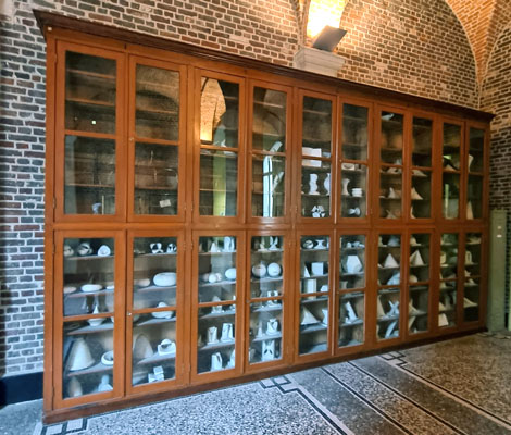
In february 2023, while working on the mathematical background and images for this page concerning Kummer surfaces, a happy coincidence occurred! On my way to a meeting with one of my former colleagues in the historical building of the "Faculty of Engineering and Architecture" at Ghent University (Belgium), I passed along the glass cabinet where are exposed a large number (at least 150) of models of mathematical surfaces and curves. When I was a student in the early 1960s, these models were already there, and we were told that they were part of the restitution payment after World War I.

As I was early for the meeting, I took a closer look and... my eyes were caught by a model of a Kummer surface!
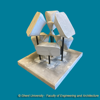
The next day my former colleague sent me an image of this model. Several curves are drawn on it. Kummer not only studied the surfaces, but also special curves on them, e.g. the intersection with the sphere and planes occuring in the definition of the surface.



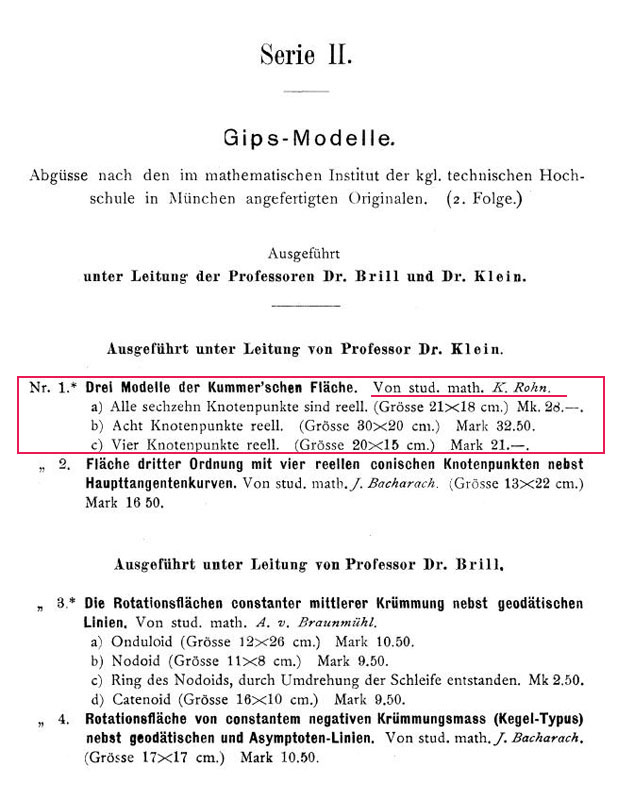
Some research on the internet led me to the catalogue (1911) of the German company "Shilling" in Leipzig. This catalogue contains numerous sketches and the description (and prices) of the large number of models they distributed. Among them are three models of a Kummer surface. The first of them is the model pictured above.


The original model apparently was located at the "Königliche Technische Hochschule" in München. It dates back to 1877. The price in 1911 was 28 Mark. In the same collection there are two other models of a Kummer surface with 4 or 8 (real) singular points. Following the catalogue, the original models are the work of the student K. Rohn. Karl Friedrich Wilhelm Rohn (1855-1920) later became a professor at the Technische Hochschule in Dresden (1887-1905) and at the University of Leipzig (1905-1920).
It seems plausible that this and other models in the collection of the Faculty of Engineering and Architecture at the Ghent University are indeed part of the restitution payment after World War I.


Kummer surfaces: mathematics

Ernst Eduard Kummer(1810-1895) was a German mathematician who made contributions to mathematics in different areas. In 1864 he discovered the family of surfaces of degree 4 that today are called "Kummer's surfaces with tetrahedral symmetry". Some Kummer surfaces contain the maximum number possible (16) of singular points for surfaces of the 4th degree.
At the end of the 19th century and even in the first half of the 20th century, there was great interest in discovering algebraic surfaces that have the maximum number possible of singular points according to their degree. The starting point mostly was symmetry. That's the reason why those images look so nice. We must not forget that in that period there were no computers to make the calculations to obtain a picture of these surfaces! The approach was very theoretical and the rare images were rather rough sketches. But, as we mentioned in the non-mathematical introduction, plaster models were produced.

Kummer surfaces are given by the equation

f ² - λ pqrs = 0
where
f(x,y,z,μ) = x²+y²+z²- μ²      
p(x,y,z) = z-1-x $\sqrt{2}$      
q(x,y,z) = z-1+x $\sqrt{2}$      
r(x,y,z) = z+1+y $\sqrt{2}$      
s(x,y,z) = z+1-y $\sqrt{2}$      
μ is a parameter and λ = (3μ² - 1)/(3 - μ²)

f(x,y,z,μ) = 0 is the equation of the sphere with radius μ centered at the origin, and p(x,y,z) = 0, q(x,yz) = 0, r(x,y,z) = 0, s(x,y,z) = 0 are the equations of the extended faces of the regular tetrahedron with vertices
(0, -$\sqrt{2}$, 1), (0, $\sqrt{2}$, 1), (-$\sqrt{2}$, 0, -1) and ($\sqrt{2}$, 0, -1).
For different values of the parameter μ, the equation of the corresponding Kummer surface is the combination of the equation of a sphere with radius μ and the equations of the four fixed planes. The combination is determined by the value of λ = (3μ² - 1)/(3 - μ²).

In some approaches a second parameter is introduced, but as it is a scaling factor, it is usually given a fixed value, here 1.

In the following image of a Kummer surface (corresponding with μ=$\sqrt{2}$), we observe the symmetry and 16 singular points (nodes). Each vertex of the tetrahedral structure in the center is a vertex of another tetrahedral structure. This allows us to say that the total number of singular points is 16. These singular points are represented by small green and red dots. Each of the 6 surrounding "basins" is attached to 2 vertices of neighbouring tetrahedral structures. As these parts extend infinitely, the surface usually is restricted to the part inside a sphere centered at the origin.



As the value of the parameter μ determines the image of the corresponding Kummer surface, it's worth to consider some special cases.
First of all we note that for λ = 0, or μ² = 1/3, the Kummer surface reduces to (twice) the sphere with radius 1/$\sqrt{3}$. For μ = 1, we get the equation of a "Roman Surface", already studied by Jakob Steiner in 1844, 20 years before Kummer discovered the surfaces that carry his name. It is called the Roman Surface because Steiner discovered it during a stay in Rome. Its equation can get different appearances, according to the orientation of the surface.

The following animations show how the (double) sphere transforms into the Roman surface as μ increases from 1/$\sqrt{3}$ to 1, and a rotating Roman surface in a different orientation.


Increasing the value of μ results in images with a totally different appearance. The Roman surface breaks up into different parts. At the very beginning we don't see what happens in the center, but four tetrahedral structures appear, and six small tubes, attached to the external vertices of these structures.



Further increasing the value of μ, we get a better view. In the center another tetrahedral structure appears. Each of its vertices is also a vertex of one of the external tetrahedral structures. The 16 different vertices are the singular points of the Kummer surface.


... and further increasing the value of μ we meet interesting situations:



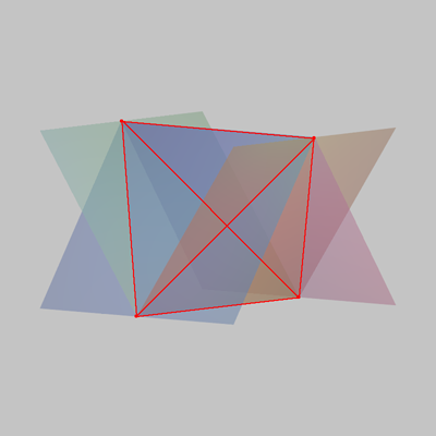
First we do have to be aware of the case μ = $\sqrt{3}$. For this value the denominator of λ equals 0. However it is easy to write the equation   f ² - λ pqrs = 0   without a denominator. It's clear that the image in the case μ = $\sqrt{3}$ is the union of the four planes that are the extended faces of the regular tetrahedron, which plays an essential role in the definition of Kummer surfaces. The vertices of the tetrahedron are the intersection points of any three of the four planes.

In this case it's better to clip the image by an appropriate box instead of by a sphere.
For a larger value for μ, the Kummer surface does not look the same as in previous cases. Only four separated tetrahedral structures remain and their vertices are the 16 singular points of the Kummer surface. Each of the four large "basins" now is attached to 3 singular points. The 4 other singular points are the top of conical surfaces.


Comparing the plaster model and the rendered surface

Finally it's interesting to compare the old plaster model I mentioned in the first part with the rendered model. I gave the Kummer surface to render the same orientation as the plaster one. It's clear that the proportion of the size of the central tetrahedral object and the four other ones depends on the value of the parameter μ. As this value isn't mentioned for the plaster model, I used μ=1.194 to obtain nearly the same configuration.
The plaster model is a solid object and the rendered one is a surface. For the plaster model the large "basins" are filled and limited by planar parts, while for the rendered image these basins are open and, as is often the case using rendering, only the part of the surface inside an appropriate sphere is rendered. The plaster model is described in catalogues and images appear in texts about Kummer surfaces, but I didn't find any information concerning the mathematical methods used in the construction.
I'm impressed by the accuracy of the plaster model. At the end of the 19th and the beginning of the 20th century it must have been a tremendous work to construct this and other models. To obtain a rendered image, numerous numerical calculations need to be done by computers and to obtain a material model 3D-printing does the job...

---

All computer images on this page were prepared using the free raytracer Povray. To combine a number of them into an animation I used Gif Movie Gear
March 2023 - updated December 2023
Herman Serras
Send Email
return to the homepage