 |
 |
Additional funding and support from the Prof. Dr. Wuytack Fund and the Department of Pure Mathematics and Computer Algebra.
| Benjamin De Leeuw |
| prof. dr. Albert Hoogewijs |
| Gent University |
| Belgium |
One of the UML diagrams is the Statechart. Invented and formalized by David Harel, it was soon integrated in the UML concept. Statecharts are used in behavior specifications. Allthough useful in the specification of complex interaction patterns, its take-up in industry is not like the other basic UML diagrams. Statecharts offer ways to define system behavior for distributed components, synchronized by event-based communication and shared memory usage. Using Statecharts to specify single component systems or even sequentially consistent distributed computations is a useless effort. Only distributed computations with very complex or non-deterministic interaction patterns are valid candidates to be modeled as UML Statecharts. Convincing examples of such complex interaction systems can be found in biological sciences. Other examples include, but are not limited to, airtraffic control systems, security intensive systems, space vehicle models, embedded systems and so on.
One of the main efforts in the computer science community is the verification of complex distributed and non-deterministic applications. With modelchecking techniques as introduced by E. Clarke, Vardi and many others, Statechart specifications can be verified to possess certain properties. Our colleague dr. Sara Van Langenhove has made an implementation which checks Statechart models for user defined properties. Look up her website here for more information on the matter.
Another important contribution of dr. Sara Van Langenhove, is her implementation of an optimization algorithm for the Statechart modelcheck computation. The algorithm makes slices of the Statechart model, depending on the properties that have to be checked. The slicing algorithm calculates ordering information on the transitions of a Statechart specification (similar to the calculation of a happens-before order on memory actions, see our other research page, Memory Model Specification and Verification for Distributed Applications). Since this is no trivial calculation, it remains to show with empirical data that the slice algorithm is indeed an optimization of the normal modelchecking algorithm.
Our work, displayed on this page, is centered around the provision of empirical and measurable data for Statechart analysis tools, like the one described in the previous paragraph. With this, we refer to the creation of Statechart test cases to empirically show the value of optimization calculations. Since Statecharts are not yet fully accepted by all branches of industry, there aren't may big and complex example Statechart specifications available to gather empirical data from. This is why we chose a different approach to gather empirical data for Statecharts: instrumented Statechart generation.
To provide instrumentation, we need to have some notion of what determines the complexity of Statecharts, from a certain viewpoint. The complexity of a third generation program is determined by analyzing the constructs offered by its context-free language grammar. We say that a context-free grammar is compositional in its application. On this page we provide an implementation which shows that the complexity of a Statechart can also validly be determined by an analysis of a generative grammar (rewrite system). More so, we show that we can specify a sort of context-free grammar for Statechart construction, just as we can for third generation programming languages, and define it as a list of compositional graphical rewrite rules on Statecharts.
As it stands now with the UML specification, the "grammar" for Statechart construction is specified as a number of graphical elements, which can be combined in a number of ways, as denoted by relevant UML metamodel-level connections (to and from Statechart construction elements). To programmers and engineers, this might seem an odd way of defining a language. It's quite fine to define language constraints, using a metamodel, for constructs which essentially denote closed sets of (static) data, but it doesn't seem to work well for constructs which are no such thing (the information shown in Statecharts, for example). Witnesses to this phenomenon are the many additional first order constraints, that have to be put on the metamodel elements for Statecharts. (Constraints of this kind are usually denoted in the Object Constraint Language, OCL).
We provide an instrumented generation process for Statecharts. Generated Statecharts are in their simplest possible form and have no pseudostates or history states. We follows the intuition displayed in the work on Scenario-based composition of Statecharts, that only a limited number of graphical element combinations make sense for Statecharts. We took the work in this area to the next level by implementing the introduced combinators as Statechart rewrite rules which transform a given Statechart into a more complex one. Taking into account only a limited number of constructs also makes most of the additional first order constraints on the Statechart metamodel unneccessary. Go to the topics Background Information and Discussion for more information on our work and that of others in this area.
Download yEd-Java Graph Editor on this page.
|
|
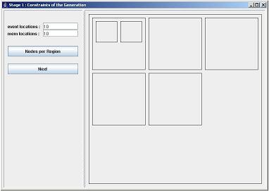
| Figure 1 |
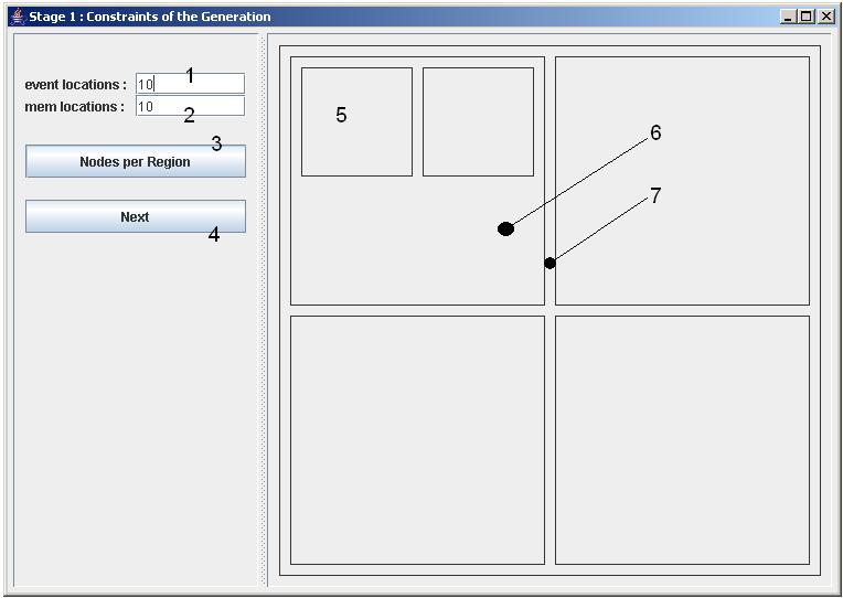
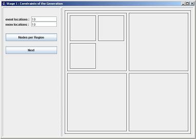
The number of memory locations (1) and the number of events (2) are relatively straightforward parameters of the generation process: the more memory or events, the more diversity in the generated actions on the transitions. Leave these fields be for the moment, but as a basic rule for their manipulation, follow the intuition that more memory locations and events make bigger Statecharts more complex in their interaction. Click a couple of times in the part of the window, labeled 5 in Fig. 1. If you click in a box (maked with 6), a new subbox is drawn and neatly positioned in the window. Starting from the configuration in the top part of Fig.1, the result would look like the lower left part of the same figure. If you already have a number of boxes specified, clicking in the whitespaces between them will add another box to the same superbox (marked with 7). The result of such an action is displayed in the lower right part of Fig. 1. Experiment a bit with this system to get the hang of it. Try to draw the boxes as displayed in Fig. 1. If you made a mistake, you'll have to restart the program, since we didn't implement an undo-function yet. Every box symbolizes a region for the generated Statechart. Every box, positioned in another box denotes a subregion for that region. All boxes together denote the region hierarchy.
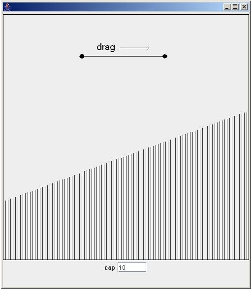
Open the Nodes per Region window by clicking on the togglebutton labeled with 3 in Fig. 1. The resulting window is displayed in Fig. 2. In this window you specify an amount vector which is scaled to a linear breath first ordering of the region hierarchy. Let's explain this. A breath first count starts with the biggest box, and goes down the hierarchy when no other boxes of the same size are found. Now count the number of boxes you have drawn (breath first) and remember it for further reference. In the top part of Fig. 1 are 7 boxes displayed, in both lower parts of Fig. 1 are 8 boxes shown. The vector, shown in the window in Fig. 2, has values between 0.0 and 1.0. Each regionbox is positioned on the X-axis of this vector, based on the breath first count of the available regions. The number of nodes or states per region is determined by taking the result of the position of the region on the X-axis, and multiplying the resulting number between 0.0 and 1.0 with the natural number, shown in the cap field. This window gives you intuitive control on the amount of nodes that is generated per region.
| ||
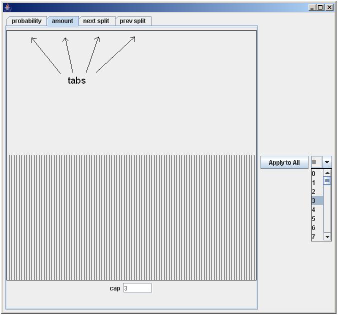
| Figure 2 |
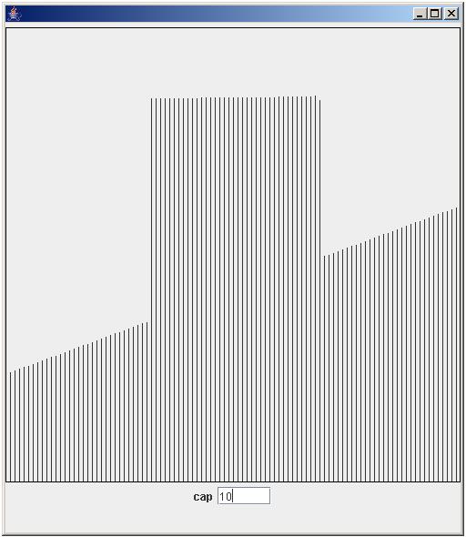
To manipulate the vector, click, drag and release the mouse somewhere in the vector window. Try to form the example vector of Fig. 2. You can use following intuition to manipulate the number nodes per regions: high values for the vector near the left end of the window, means that the top level region and its direct subregions have a larger amount of nodes available, high values for the vector near the right end of the window, denotes many available nodes for the deeper regions in the region hierarchy. As an exercise, use your breath first count of Fig. 1 to determine the expected number of nodes for each of the 7 or 8 regions available. The top-level region has 3 nodes available, the deepest region(s) has 5 nodes available. The middle regions have either 4 nodes (left part of Fig.2) or 8 nodes (right part of Fig.2) available. The cap textfield shows the absolute maximum of nodes per region. Now, for this tutorial, try to draw a vector with maximum nodes (10) for every region. Your vector should fill the entire window. Close the Nodes per Region window by pressing the close icon, or by toggling the button, labeled 3 in Fig. 1. Additional changes to the amount vector can be made, as long as your don't press the Next button (labeled 4 in Fig. 1).
Press Next to get to the window, displayed in Fig. 3. This part of our Statechart generation constraining is entirely optional. If you plan on manually generate a complete Statechart, you don't have to do anything here, just press the Start button (labeled 4 in Fig. 3) to start the generation process. If you plan on letting the generator do some of the work for you, this window is your key to letting the generator do the things you desire. Let us therefore discuss the window in Fig. 3 in more detail.
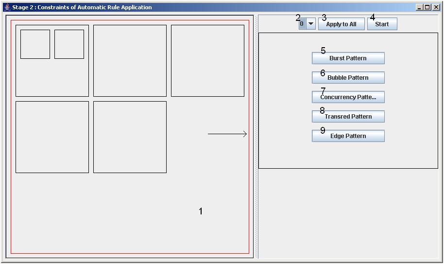 |
| Figure 3 |
The left part of the window, labeled 1 in Fig. 3, displays the region hierarchy. It can no longer be manipulated. Every region now has a region number and a box. Every region also has five patterns which guide the Statechart generation process. These patterns are manipulated in the right part of the window. Select a region from the region hierarchy with the combobox labeled with 2 in Fig. 3. The current regionbox is displayed in red, as pointed out by an arrow in Fig. 3. Use the button Apply to All, labeled 3 in Fig. 3, to apply the patterns of the current region to all other regions. Use the Start button to quit this window and start the generation process. Clicking on one of the togglebuttons, labeled 5 to 9, brings up other windows, where you can change the regional generation patterns. The different windows have different effects but all behave in a very similar way. The basic controls for these windows are the same as the Nodes per Region window in Fig. 2. Click, drag, release to draw the vectors, use the cap field to denote the absolute maximum where necessary. A pattern consists of multiple (2 to 4) of these windows of Fig. 2. We grouped them in a tabbed pane, per pattern. An example of such a window is given in Fig. 4. Press the Bubble Pattern togglebutton for this window to appear.
 |
| Figure 4 |
As already said before, the controls for this kind of window are just the same as those for the window in Fig. 2. The tabs are a new element, as is the combobox with numbers from 0 to 99. The combobox controls the next split and prev split tabs. One single split pattern, is a vector like before, which controls the redistribution of incoming and outgoing transitions or edges for a certain node during the application of certain rewrite rules (see below). A split pattern for all nodes in one region is a vector of single split pattern vectors, hence a vector of vectors. Explained in a 3-dimensional way: the X-axis of each split pattern is the X-axis you see displayed in the next split and prev split tabs, the Y-axis is controlled by the combobox from 0 to 99 (100 discrete positions, just as the X-axis), and the Z-axis is the composition of all 100 vectors and displays a result between 0.0 and 1.0 for all 10,000 positions. The Apply to All button copies the current next split and prev split patterns to each of the 99 other positions on the Y-axis. The other two tabs (probability and amount) are not controlled by the combobox and work on the current region as a whole.
Following table gives an overview of all tabs for each pattern and what they mean:
| Pattern | Tabs | ||||||||
|---|---|---|---|---|---|---|---|---|---|
| burst |
|
||||||||
| bubble |
|
||||||||
| concurrency |
|
||||||||
| transreduction |
|
||||||||
| edge |
|
Remark on this table that some rewrite rules are applied at edges, while others are applied to nodes. The ordering, we refer to, to scale the vectors to, is again a breadth first count (just like the region hierarchy count). Things you do at the left side of these pattern windows, have an effect on the nodes or edges nearest to the regional start edge. Things you do at the right side have an effect on nodes or edges that lie near the furthest terminating path ends. For more information on the patterns refer to this section.
As an easy exercise, set the probability of all patterns for all regions (use the Apply to All button) to around 75%. Set the amount for all patterns except the Edge Pattern for all regions to 2. Set the list length in the Edge Pattern to 3 and the ratio mem event in the middle (evenly matched event and memory operations in the action lists). Leave all split patterns as they are by default. Click on the Start button to proceed to the generation screen, displayed in Fig. 5.
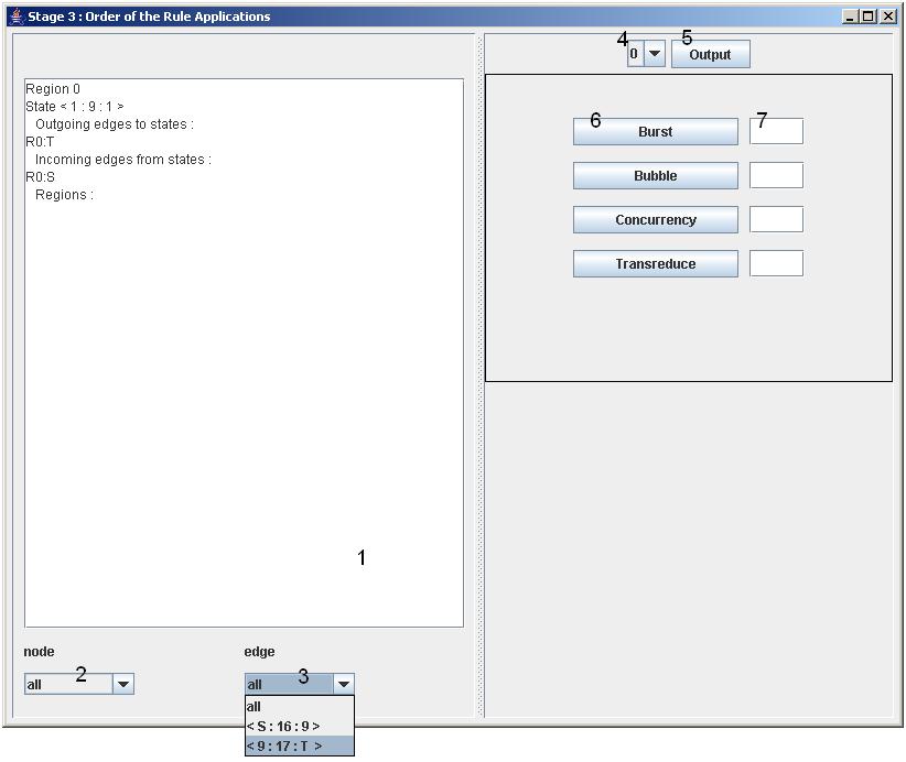 |
| Figure 5 |
The part of the window, labeled with 1 in Fig. 5 shows the current region and its contents in a very simple textual format. The four rewrite rules can be applied to all nodes or edges simultaneously, using probability, amount and if necessary the split pattern constraints of the previous window (Fig. 3). Patterns can also be applied to one node or edge at a time, by selecting nodes or edges with the comboboxes labeled 2 and 3 in Fig. 5. As soon as more regions are connected to the Statechart, due to Concurrency rule application, new regionnumbers will become available in the combobox on the right hand side of the window, labeled 4 in Fig. 5. Select new regions to work on with this combobox. Remark that the current region number is also displayed in the textfield, marked with 1 in Fig. 5. Clicking the Output button, marked with 5 in Fig. 5, will close the generation process and produce the output.
Before we do this, we should however, do something with the basic statechart, displayed in the only connected region (the top-level regionbox of the region hierarchy). We are going to rewrite it, using the four rules, displayed at the right, and marked 6 in Fig.5. Next to each rule button is a textfield, labeled 7 in Fig. 5.
We start with the basic operations. Select the only node present in the region, with the combobox labeled 2 in Fig. 5. Type "3" in the textfield next to the Bubble button and afterwards press that button. There should now be four nodes present in your current (top-level) region, connected in a circular fashion. This way is the most constrained way of applying a rewrite rule: you determine the node or edge to which the rule is applied, and determine the amount of nodes or regions that is added (namely, the number written in the textfields next to the rule buttons). The only thing left to patterns is the repartitioning of the incoming and outgoing transitions for the node or edge under consideration, using a split pattern.
For the semi-automatic operations, select one of the edges that has no "S" in its name, with the combobox labeled 3 in Fig. 5. Delete everything that is in the textfield next to the Burst button, or put something that does not look like an integer in it. Press the Burst button. If you constructed the patterns as suggested by this tutorial, you should see two new nodes added to the region, connected in a diamond shape fashion to the source and destination of your chosen edge. (Draw the current configuration of your region on a piece of paper if you like. For a more in-depth discussion of the rewrite rules, refer to this section.) The rule is applied to your chosen edge or node, but the amount and the split patterns are determined by your input in the previous window (Fig. 3).
For the fully automatic operations, select all as node or edge in the combobox labeled 2 or 3 in Fig. 5. You just start pressing buttons, and the relevant rewrite rules are applied to all nodes or edges, with probability, amount and split patterns as specified in the previous window (Fig. 3). If your buttons blank out during this process, it means that you are out of nodes for that region, or more generally, that there is no other valid application of that rule in the current region.
As soon as you have connected more than one region, you can start the process all over again for that new region, by selecting it with the combobox labeled 4 in Fig. 5. Regions can be worked on until satisfied or out of options. As an exercise, you can for example create a Statechart with two concurrent regions, with in each region a cycle of three nodes. (Use the Concurrency rule once with parameter "2", afterwards, use in both new regions the Bubble rule with parameter "3".) Press the Output button when finished. The resulting window is displayed in Fig. 6.
 |
| Figure 6 |
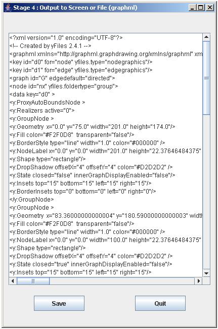
The output of our program is a graphml representation of the Statechart graph. graphml is an XML-based language for hierarchical graph representation. It is a textual language, which can be manipulated with any text editor, as desired. It is also XML, so you can use an XML-editor, if you like. Most importantly the freeware tool yEd can be used to read the graphml files and display their content (graphs) on the screen. In the window shown in Fig. 6, you can save the (edited) text with the Save button. A standard file dialog window pops up and you are prompted to select a file. If you select a file, it is overwritten without warning, so be careful! If you want to create a new file, type in the relevant field the filename with the extension ".graphml" or ".txt", as desired. Quit the program if finished. Use yEd to read the created file.
If you experienced problems, or can't get yEd installed, look up the examples below for some results of the
Statechart generation process.
Statechart Rewrite Rules
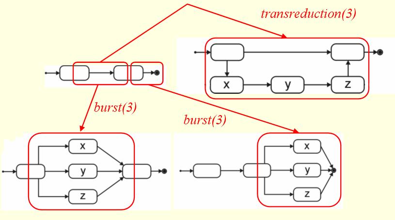
Each application of a rewrite rule replaces an edge or a node with a more complex construct. Incoming and outgoing edges are detached and
reattached to different nodes in this more complex construct. Figure 7 and 8 display the different rewrite rules graphically, for a certain
amount.
 |
| Figure 7 |
The burst rule is an edge-based rule. It replaces an edge, with a number of nodes, connected in diamond shape fashion to the source and destination of this edge. The rule only requires an amount parameter. See Fig. 7 for more details.
The transreduction rule is an edge-based rule. It leaves the edge and constructs a transitive reduction path from the source to the destination of the edge under consideration. Incoming edges of the source node and outgoing edges of the destination node are redistributed among the original nodes and the newly created ones, and this according to a prev split and next split pattern respectively. Start edges and termination edges are not redistributed, but stay attached to the original nodes. The transreduction rule cannot be applied to a termination edge. Figure 7 displays this process.
 |
| Figure 8 |
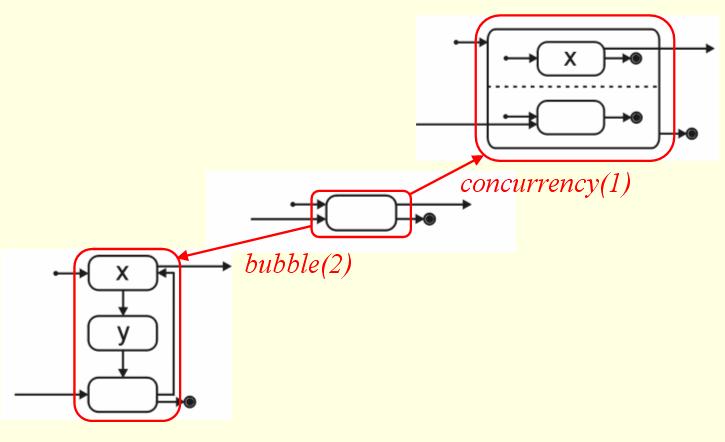
The bubble rule is a node-based rule. It attaches a number of nodes to the original node in a circular fashion. The amount of nodes to be added by the rule, is specified by an amount parameter. All incoming and outgoing edges of the original node are redistributed among the original node and the newly created ones, guided by prev split and next split patterns. The process is shown in Fig. 8.
The concurrency rule creates a number of subregions in the node it rewrites. The number of regions is denoted by the amount parameter, and
the regions are picked from the children of the current region in the region hierarchy. Edges are redistributed to the original node itself
and the only node in the newly created regions. Start and termination edges are left attached to the original outer node. The process is illustrated
in Fig. 8.
Details of the Statechart Generation Control Mechanisms
As already explained in the tutorial there are essentially three kinds of patterns to guide the Statechart generation process:
 |
| Figure 9 |
The X-axis of the first two kinds of patterns is evenly partitioned. Each element that requires a result, is assigned to one such partition. This is shown by vertical red lines in Fig. 9. Next, the mean of each partition is calculated and this gives the final result for each element. In Fig. 9 this is shown by horizontal lines for each partition.
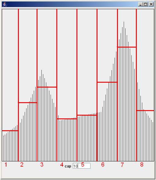
The third pattern behaves a bit differently, and the process is shown in Fig. 10. The X-axis of the pattern is again divided evenly among the result requiring constructs (nodes), as depicted in Fig. 10 by red vertical lines. Given a number of elements to be partitioned (incoming or outgoing edges), the result is an array which denotes the different partitions of the given elements for each result requesting construct.
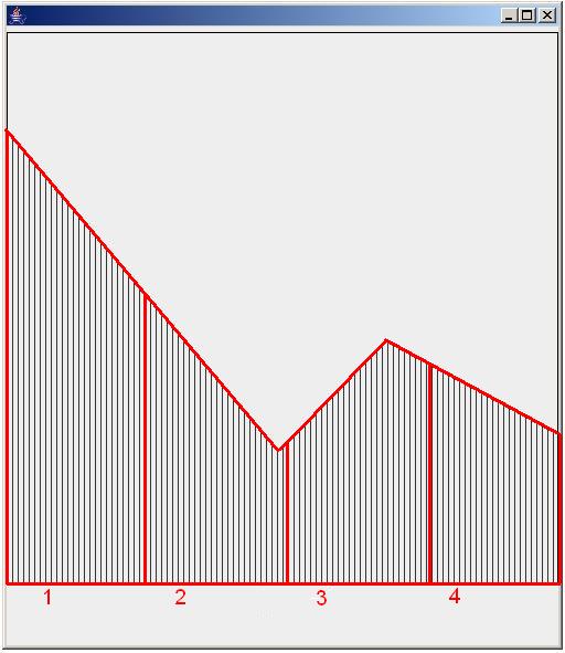 |
| Figure 10 |
If for example 10 edges need to be distributed among 4 nodes (as in Fig. 10), the area of each node is scaled to the total area (marked by red contours), and depending on the fraction of this total area, a number of elements is taken. The result is an array of four positions, which sums up to 10, and which denotes the distribution of the 10 edges among 4 nodes.
Split patterns are defined as vectors of vectors with 100 positions. If we need a split pattern for a specific node, we use the same technique as in Fig. 9: we divide the 100 positions evenly among the result requesting elements, and calculate the mean split pattern for each result requesting element. The calculation of the mean split pattern is a variation on the calculation of the mean value as shown in Fig. 9 (vectors are now middled out instead of values). Remark that if the Apply to All button was used to define the 100 split patterns the mean split pattern calculation has no effect (you always get the same vector for that region, namely the one you drew and applied to all others).
In the case of memory actions (reads and writes), the exact condition under which a guard is fulfilled is not generated, since this would make the action language at least as complex as a normal programming language. The intended meaning of the guards on our generated Statecharts is this: a guard like [read a] means anything from a > 5 to sqrt(a) + 3 == 5, for example. Hence, we only denote which memory value is read to check the guard, not the actual value of the read. A memory write in an action list symbolizes anything of the form a = ... (any assignment of the designated memory location).
Event write actions in the action list symbolize the generation of events by concurrently communicating Statechart regions. They fulfill triggers on neighbouring regions' transitions, just like in normal Statecharts.
The number of locations for event and memory operations is constrained by the user, in the opening screen of the program (see tutorial, Fig. 1 for more information). The number of event locations is distributed among all concurrent regions. These sets determine the events that can be generated by that region. Recursively we calculate which regions can be triggered by the different event write actions. These determine the triggers that can be generated in those regions. Given a certain event probability and action list composition, triggers and event writes are generated on the transitions of certain concurrent regions. Remark that not all event write actions will be able to connect to triggers in neighbouring regions (for example, if there are no triggers generated in those neighbouring regions). Because event based communication is non-deterministic by nature, this is not a problem.
At the beginning of the edge label generation process, all available memory locations (see tutorial, Fig. 1 for more information) are stored in an unused memory list. All edges are counted in a partial breadth first order. Given a certain memory probability and action list composition, when an action list with a memory action is generated, that memory location goes to the used memory list, after all other branches (edges) of that point in the partial order are generated. Guards are generated from this used memory list. As long as the used memory list is empty, no guards are generated. This way we guarantee that every memory location is first written, before it is read.
The generated Statecharts are non-deterministic because it can happen that more than one outgoing edge is labeled with the same trigger and/or guard.
Using yEd to Display the Generated Statecharts
To download yEd-Java Graph Editor, use this link. yEd is a graph editor, supporting
lots of input formats for graphs (.ygf,.graphml,.graphmlz,.gml,.xgml,.thf). Most interesting feature of this program are its graph node positioning algoritms.
With yEd installed, double click the generated .graphml file or open it using the yEd menu. Position the nodes of the generated Statechart with the Layout menu. For the best effect, use the Hierarchical>Classic layout algorithm. Afterwards select the layout Edge Router>Orthogonal for the edge positioning. For long edge labels this layout is still not the ideal, but it is to be expected that new layouts will be made available to the program over time. Save your graphs or export them to an image (.html,.jpeg,.pdf) for further use. See the examples for some results.
| graphml | html | Description |
|---|---|---|
| Example 1 | Example 1 | industrial size Statechart with many interactions |
| Example 2 | Example 2 | industrial size Statechart with many interactions |
| Example 3 | Example 3 | illustration of a disconnected Statechart (bug, to be resolved) |
| Example 4 | Example 4 | simple Statechart with burst and concurrency applications |
| Example 5 | Example 5 | simple Statechart with concurrent redistribution of edges |
| Example 6 | Example 6 | simple Statechart with burst, bubble and concurrency applications |