dotty which is a sophisticated graph drawing program. We also provide DrawDiagramWithNeato to make a diagram with straight lines, using neato. Here is what the output looks like with the standard DrawDiagram command: 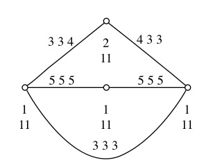
In this chapter we provide some simple examples of the use of FinInG.
In this example, we consider a hyperoval of the projective plane PG(2,4), that is, six points no three collinear. We will construct such a hyperoval by exploring a bit the particular properties of the projective plane PG(2,4). The projective plane is initalised, its points are computed and listed; then a standard frame is constructed, of which we may assume that it is a subset of the hyperoval. Finally, the stabiliser group of the hyperoval is computed, and it is checked that this group is isomorphic with the symmetric group on six elements.
gap> pg := ProjectiveSpace(2,4);
ProjectiveSpace(2, 4)
gap> points := Points(pg);
<points of ProjectiveSpace(2, 4)>
gap> pointslist := AsList(points);
[ <a point in ProjectiveSpace(2, 4)>, <a point in ProjectiveSpace(2, 4)>,
  <a point in ProjectiveSpace(2, 4)>, <a point in ProjectiveSpace(2, 4)>,
  <a point in ProjectiveSpace(2, 4)>, <a point in ProjectiveSpace(2, 4)>,
  <a point in ProjectiveSpace(2, 4)>, <a point in ProjectiveSpace(2, 4)>,
  <a point in ProjectiveSpace(2, 4)>, <a point in ProjectiveSpace(2, 4)>,
  <a point in ProjectiveSpace(2, 4)>, <a point in ProjectiveSpace(2, 4)>,
  <a point in ProjectiveSpace(2, 4)>, <a point in ProjectiveSpace(2, 4)>,
  <a point in ProjectiveSpace(2, 4)>, <a point in ProjectiveSpace(2, 4)>,
  <a point in ProjectiveSpace(2, 4)>, <a point in ProjectiveSpace(2, 4)>,
  <a point in ProjectiveSpace(2, 4)>, <a point in ProjectiveSpace(2, 4)>,
  <a point in ProjectiveSpace(2, 4)> ]
gap> Display(pointslist[1]);
 . . 1
Now we may assume that our hyperoval contains the fundamental frame.
gap> frame := [[1,0,0],[0,1,0],[0,0,1],[1,1,1]]*Z(2)^0;
[ [ Z(2)^0, 0*Z(2), 0*Z(2) ], [ 0*Z(2), Z(2)^0, 0*Z(2) ],
  [ 0*Z(2), 0*Z(2), Z(2)^0 ], [ Z(2)^0, Z(2)^0, Z(2)^0 ] ]
gap> frame := List(frame,x -> VectorSpaceToElement(pg,x));
[ <a point in ProjectiveSpace(2, 4)>, <a point in ProjectiveSpace(2, 4)>,
  <a point in ProjectiveSpace(2, 4)>, <a point in ProjectiveSpace(2, 4)> ]
Alternatively, we could use:
gap> frame := StandardFrame( pg );
[ <a point in ProjectiveSpace(2, 4)>, <a point in ProjectiveSpace(2, 4)>,
  <a point in ProjectiveSpace(2, 4)>, <a point in ProjectiveSpace(2, 4)> ]
There are six secant lines to this frame (``four choose two''). So we put together these secant lines from the pairs of points of this frame.
gap> pairs := Combinations(frame,2);
[ [ <a point in ProjectiveSpace(2, 4)>, <a point in ProjectiveSpace(2, 4)> ],
  [ <a point in ProjectiveSpace(2, 4)>, <a point in ProjectiveSpace(2, 4)> ],
  [ <a point in ProjectiveSpace(2, 4)>, <a point in ProjectiveSpace(2, 4)> ],
  [ <a point in ProjectiveSpace(2, 4)>, <a point in ProjectiveSpace(2, 4)> ],
  [ <a point in ProjectiveSpace(2, 4)>, <a point in ProjectiveSpace(2, 4)> ],
  [ <a point in ProjectiveSpace(2, 4)>, <a point in ProjectiveSpace(2, 4)> ] ]
gap> secants := List(pairs,p -> Span(p[1],p[2]));
[ <a line in ProjectiveSpace(2, 4)>, <a line in ProjectiveSpace(2, 4)>,
  <a line in ProjectiveSpace(2, 4)>, <a line in ProjectiveSpace(2, 4)>,
  <a line in ProjectiveSpace(2, 4)>, <a line in ProjectiveSpace(2, 4)> ]
By a counting argument, it is known that the frame of PG(2,4) completes uniquely to a hyperoval.
gap> leftover := Filtered(pointslist,t->not ForAny(secants,s->t in s));
[ <a point in ProjectiveSpace(2, 4)>, <a point in ProjectiveSpace(2, 4)> ]
gap> hyperoval := Union(frame,leftover);
[ <a point in ProjectiveSpace(2, 4)>, <a point in ProjectiveSpace(2, 4)>,
  <a point in ProjectiveSpace(2, 4)>, <a point in ProjectiveSpace(2, 4)>,
  <a point in ProjectiveSpace(2, 4)>, <a point in ProjectiveSpace(2, 4)> ]
This hyperoval has the symmetric group on six symbols as its stabiliser, which can easily be calculated:
gap> g := CollineationGroup(pg);
The FinInG collineation group PGammaL(3,4)
gap> stab := Stabilizer(g,Set(hyperoval),OnSets);
<projective collineation group of size 720>
gap> StructureDescription(stab);
"S6"
Here we see how the lines of a projective plane PG(2,q2 ) meet a hermitian curve. It is well known that every line meets in either 1 or q+1 points.
gap> h:=HermitianPolarSpace(2, 7^2);
H(2, 7^2)
gap> pg := AmbientSpace( h );
ProjectiveSpace(2, 49)
gap> lines := Lines( pg );
<lines of ProjectiveSpace(2, 49)>
gap> curve := AsList( Points( h ) );;
gap> Size(curve);
344
gap> Collected( List(lines, t -> Number(curve, c-> c in t)));
[ [ 1, 344 ], [ 8, 2107 ] ]
In this example, we embed W(3,3) in W(5,3).
gap> w3 := SymplecticSpace(3, 3);
W(3, 3)
gap> w5 := SymplecticSpace(5, 3);
W(5, 3)
gap> pg := AmbientSpace( w5 );
ProjectiveSpace(5, 3)
gap> solids := ElementsOfIncidenceStructure(pg, 4);
<solids of ProjectiveSpace(5, 3)>
gap> iter := Iterator( solids );
<iterator>
gap> perp := PolarityOfProjectiveSpace( w5 );
<polarity of PG(5, GF(3)) >
gap> solid := NextIterator( iter );
<a solid in ProjectiveSpace(5, 3)>
gap> solid^perp;
<a line in ProjectiveSpace(5, 3)>
gap> em := NaturalEmbeddingBySubspace( w3, w5, solid );
<geometry morphism from <Elements of W(3, 3)> to <Elements of W(5, 3)>>
gap> points := Points( w3 );
<points of W(3, 3)>
gap> points2 := ImagesSet(em, AsSet(points));;
gap> ForAll(points2, x -> x in solid);
true
A spread of W(5,q) is a set of q3+1 planes which partition the points of W(5,q). Here we enumerate all spreads of W(5,3) which have a set-wise stabiliser of order a multiple of 13.
gap> w := SymplecticSpace(5, 3);
W(5, 3)
gap> g := IsometryGroup(w);
PSp(6,3)
gap> syl := SylowSubgroup(g, 13);
<projective collineation group of size 13>
gap> planes := Planes( w );
<planes of W(5, 3)>
gap> points := Points( w );
<points of W(5, 3)>
gap> orbs := Orbits(syl, planes , OnProjSubspaces);;
gap> IsPartialSpread := x -> Number(points, p ->
>          ForAny(x, i-> p in i)) = Size(x)*13;;
gap> partialspreads := Filtered(orbs, IsPartialSpread);;
gap> Length(partialspreads);
8
gap> 13s := Filtered(partialspreads, i -> Size(i) = 13);;
gap> Length(13s);
6
gap> 13s[1];
[ <a plane in W(5, 3)>, <a plane in W(5, 3)>, <a plane in W(5, 3)>,
  <a plane in W(5, 3)>, <a plane in W(5, 3)>, <a plane in W(5, 3)>,
  <a plane in W(5, 3)>, <a plane in W(5, 3)>, <a plane in W(5, 3)>,
  <a plane in W(5, 3)>, <a plane in W(5, 3)>, <a plane in W(5, 3)>,
  <a plane in W(5, 3)> ]
gap> 26s := List(Combinations(13s,2), Union);;
gap> two := Union(Filtered(partialspreads, i -> Size(i) = 1));;
gap> good26s := Filtered(26s, x->IsPartialSpread(Union(x, two)));;
gap> spreads := List(good26s, x->Union(x, two));;
gap> Length(spreads);
5
In this example, we construct the unique ovoid of the parabolic quadric Q(6,3), first discovered by Patterson, but for which was given a nice construction by E. E. Shult. We begin with the ``sums of squares'' quadratic form over GF(3) and the associated polar space.
gap> id := IdentityMat(7, GF(3));;
gap> form := QuadraticFormByMatrix(id, GF(3));
< quadratic form >
gap> ps := PolarSpace( form );
<polar space in ProjectiveSpace(
6,GF(3)): x_1^2+x_2^2+x_3^2+x_4^2+x_5^2+x_6^2+x_7^2=0 >
The construction of the ovoid (a la Shult):
gap> psl32 := PSL(3,2);
Group([ (4,6)(5,7), (1,2,4)(3,6,5) ])
gap> reps:=[[1,1,1,0,0,0,0], [-1,1,1,0,0,0,0],
> [1,-1,1,0,0,0,0], [1,1,-1,0,0,0,0]]*Z(3)^0;
[ [ Z(3)^0, Z(3)^0, Z(3)^0, 0*Z(3), 0*Z(3), 0*Z(3), 0*Z(3) ],
  [ Z(3), Z(3)^0, Z(3)^0, 0*Z(3), 0*Z(3), 0*Z(3), 0*Z(3) ],
  [ Z(3)^0, Z(3), Z(3)^0, 0*Z(3), 0*Z(3), 0*Z(3), 0*Z(3) ],
  [ Z(3)^0, Z(3)^0, Z(3), 0*Z(3), 0*Z(3), 0*Z(3), 0*Z(3) ] ]
gap> ovoid := Union( List(reps, x-> Orbit(psl32, x, Permuted)) );;
gap> ovoid := List(ovoid, x -> VectorSpaceToElement(ps, x));;
We check that this is indeed an ovoid...
gap> planes := AsList( Planes( ps ) );;
#I  Computing collineation group of canonical polar space...
gap> ForAll(planes, p -> Number(ovoid, x -> x in p) = 1);
true
The stabiliser is interesting since it yields the embedding of Sp(6,2) in PO(7,3). To efficiently compute the set-wise stabiliser, we refer to the induced permutation representation.
gap> g := IsometryGroup( ps );
<projective collineation group of size 9170703360 with 2 generators>
gap> stabovoid := SetwiseStabilizer(g, OnProjSubspaces, ovoid)!.setstab;
#I  Computing adjusted stabilizer chain...
<projective collineation group with 12 generators>
gap> DisplayCompositionSeries(stabovoid);
G (size 1451520)
 | B(3,2) = O(7,2) ~ C(3,2) = S(6,2)
1 (size 1)
gap> OrbitLengths(stabovoid, ovoid);
[ 28 ]
gap> IsTransitive(stabovoid, ovoid);
true
In this example, we construct a classical elation generalised quadrangle from a q-clan, and we see that the associated BLT-set is a conic.
gap> f := GF(3);
GF(3)
gap> id := IdentityMat(2, f);;
gap> clan := List( f, t -> t*id );;
gap> IsqClan( clan, f );
true
gap> clan := qClan(clan, f);
<q-clan over GF(3)>
gap> egq := EGQByqClan( clan );
#I  Computed Kantor family. Now computing EGQ...
#I  Computing points from Kantor family...
#I  Computing lines from Kantor family...
<EGQ of order [ 9, 3 ] and basepoint 0>
gap> elations := ElationGroup( egq );
<matrix group of size 243 with 8 generators>
gap> points := Points( egq );
<points of <EGQ of order [ 9, 3 ] and basepoint 0>>
gap> p := Random(points);
<a point of a Kantor family>
gap> x := Random(elations);
[ [ Z(3)^0, Z(3), Z(3)^0, Z(3) ], [ 0*Z(3), Z(3)^0, 0*Z(3), 0*Z(3) ],
  [ 0*Z(3), 0*Z(3), Z(3)^0, Z(3)^0 ], [ 0*Z(3), 0*Z(3), 0*Z(3), Z(3)^0 ] ]
gap> OnKantorFamily(p,x);
<a point of a Kantor family>
gap> orbs := Orbits( elations, points, OnKantorFamily);;
gap> Collected(List( orbs, Size ));
[ [ 1, 1 ], [ 9, 4 ], [ 243, 1 ] ]
gap> blt := BLTSetByqClan( clan );
[ <a point in Q(4, 3): -x_1*x_5-x_2*x_4+x_3^2=0>,
  <a point in Q(4, 3): -x_1*x_5-x_2*x_4+x_3^2=0>,
  <a point in Q(4, 3): -x_1*x_5-x_2*x_4+x_3^2=0>,
  <a point in Q(4, 3): -x_1*x_5-x_2*x_4+x_3^2=0> ]
gap> q4q := AmbientGeometry( blt[1] );
Q(4, 3): -x_1*x_5-x_2*x_4+x_3^2=0
gap> span := Span( blt );
<a plane in ProjectiveSpace(4, 3)>
gap> ProjectiveDimension( span );
2
We will construct an elation generalised quadrangle directly from the Kantor-Knuth semifield q-clan and also via its corresponding BLT-set. The q-clan in question here are the set of matrices Ct of the form
|
gap> q := 9;
9
gap> f := GF(q);
GF(3^2)
gap> squares := AsList(Group(Z(q)^2));
[ Z(3)^0, Z(3), Z(3^2)^2, Z(3^2)^6 ]
gap> n := First(GF(q), x -> not IsZero(x) and not x in squares);
Z(3^2)
gap> sigma := FrobeniusAutomorphism( f );
FrobeniusAutomorphism( GF(3^2) )
gap> zero := Zero(f);
0*Z(3)
gap> qclan := List(GF(q), t -> [[t, zero], [zero,-n * t^sigma]] );
[ [ [ 0*Z(3), 0*Z(3) ], [ 0*Z(3), 0*Z(3) ] ],
  [ [ Z(3^2), 0*Z(3) ], [ 0*Z(3), Z(3)^0 ] ],
  [ [ Z(3^2)^5, 0*Z(3) ], [ 0*Z(3), Z(3) ] ],
  [ [ Z(3)^0, 0*Z(3) ], [ 0*Z(3), Z(3^2)^5 ] ],
  [ [ Z(3^2)^2, 0*Z(3) ], [ 0*Z(3), Z(3^2)^3 ] ],
  [ [ Z(3^2)^3, 0*Z(3) ], [ 0*Z(3), Z(3^2)^6 ] ],
  [ [ Z(3), 0*Z(3) ], [ 0*Z(3), Z(3^2) ] ],
  [ [ Z(3^2)^7, 0*Z(3) ], [ 0*Z(3), Z(3^2)^2 ] ],
  [ [ Z(3^2)^6, 0*Z(3) ], [ 0*Z(3), Z(3^2)^7 ] ] ]
gap> IsqClan( qclan, f );
true
gap> qclan := qClan(qclan , f);
<q-clan over GF(3^2)>
gap> egq1 := EGQByqClan( qclan);
#I  Computed Kantor family. Now computing EGQ...
#I  Computing points from Kantor family...
#I  Computing lines from Kantor family...
<EGQ of order [ 81, 9 ] and basepoint 0>
gap> blt := BLTSetByqClan( qclan );
[ <a point in Q(4, 9): -x_1*x_5-x_2*x_4+Z(3^2)^5*x_3^2=0>,
  <a point in Q(4, 9): -x_1*x_5-x_2*x_4+Z(3^2)^5*x_3^2=0>,
  <a point in Q(4, 9): -x_1*x_5-x_2*x_4+Z(3^2)^5*x_3^2=0>,
  <a point in Q(4, 9): -x_1*x_5-x_2*x_4+Z(3^2)^5*x_3^2=0>,
  <a point in Q(4, 9): -x_1*x_5-x_2*x_4+Z(3^2)^5*x_3^2=0>,
  <a point in Q(4, 9): -x_1*x_5-x_2*x_4+Z(3^2)^5*x_3^2=0>,
  <a point in Q(4, 9): -x_1*x_5-x_2*x_4+Z(3^2)^5*x_3^2=0>,
  <a point in Q(4, 9): -x_1*x_5-x_2*x_4+Z(3^2)^5*x_3^2=0>,
  <a point in Q(4, 9): -x_1*x_5-x_2*x_4+Z(3^2)^5*x_3^2=0>,
  <a point in Q(4, 9): -x_1*x_5-x_2*x_4+Z(3^2)^5*x_3^2=0> ]
gap> egq2 := EGQByBLTSet( blt );
#I  No intertwiner computed. One of the polar spaces must have a collineation group computed
#I  Now embedding dual BLT-set into W(5,q)...
#I  Computing points(1) of Knarr construction...
#I  Computing lines(1) of Knarr construction...
#I  Computing points(2) of Knarr construction...
#I  Computing lines(2) of Knarr construction...please wait
#I  Computing elation group...
<EGQ of order [ 81, 9 ] and basepoint [ Z(3)^0, 0*Z(3), 0*Z(3), 0*Z(3),
   0*Z(3), 0*Z(3) ]>
Here we look at a particular flag-transitive geometry constructed from four subgroups of PSL(2,11), and we construct the diagram for this geometry. To view this diagram, you need to either use a postscript viewer or a dotty viewer (such as GraphViz).
gap> g := PSL(2,11);
Group([ (3,11,9,7,5)(4,12,10,8,6), (1,2,8)(3,7,9)(4,10,5)(6,12,11) ])
gap> g1 := Group([ (1,2,3)(4,8,12)(5,10,9)(6,11,7), (1,2)(3,4)(5,12)(6,11)(7,10)(8,9) ]);
Group([ (1,2,3)(4,8,12)(5,10,9)(6,11,7), (1,2)(3,4)(5,12)(6,11)(7,10)(8,9) ])
gap> g2 := Group([ (1,2,7)(3,9,4)(5,11,10)(6,8,12), (1,2)(3,4)(5,12)(6,11)(7,10)(8,9) ]);
Group([ (1,2,7)(3,9,4)(5,11,10)(6,8,12), (1,2)(3,4)(5,12)(6,11)(7,10)(8,9) ])
gap> g3 := Group([ (1,2,11)(3,8,7)(4,9,5)(6,10,12), (1,2)(3,12)(4,11)(5,10)(6,9)(7,8) ]);
Group([ (1,2,11)(3,8,7)(4,9,5)(6,10,12), (1,2)(3,12)(4,11)(5,10)(6,9)(7,8) ])
gap> g4 := Group([ (1,2,11)(3,8,7)(4,9,5)(6,10,12), (1,2)(3,10)(4,9)(5,8)(6,7)(11,12) ]);
Group([ (1,2,11)(3,8,7)(4,9,5)(6,10,12), (1,2)(3,10)(4,9)(5,8)(6,7)(11,12) ])
gap> cg := CosetGeometry(g, [g1,g2,g3,g4]);
CosetGeometry( Group( [ ( 3,11, 9, 7, 5)( 4,12,10, 8, 6),
  ( 1, 2, 8)( 3, 7, 9)( 4,10, 5)( 6,12,11) ] ) )
gap> SetName(cg, "Gamma");
gap> ParabolicSubgroups(cg);
[ Group([ (1,2,3)(4,8,12)(5,10,9)(6,11,7), (1,2)(3,4)(5,12)(6,11)(7,10)(8,9)
     ]),
  Group([ (1,2,7)(3,9,4)(5,11,10)(6,8,12), (1,2)(3,4)(5,12)(6,11)(7,10)(8,9)
     ]),
  Group([ (1,2,11)(3,8,7)(4,9,5)(6,10,12), (1,2)(3,12)(4,11)(5,10)(6,9)(7,8)
     ]),
  Group([ (1,2,11)(3,8,7)(4,9,5)(6,10,12), (1,2)(3,10)(4,9)(5,8)(6,7)(11,12)
     ]) ]
gap> BorelSubgroup(cg);
Group(())
gap> AmbientGroup(cg);
Group([ (3,11,9,7,5)(4,12,10,8,6), (1,2,8)(3,7,9)(4,10,5)(6,12,11) ])
gap> type2 := ElementsOfIncidenceStructure( cg, 2 );
<elements of type 2 of Gamma>
gap> IsFlagTransitiveGeometry( cg );
true
gap> DrawDiagram( DiagramOfGeometry(cg), "PSL211");
The output of this example uses dotty which is a sophisticated graph drawing program. We also provide DrawDiagramWithNeato to make a diagram with straight lines, using neato. Here is what the output looks like with the standard DrawDiagram command:
generated by GAPDoc2HTML